Inferring magnetic geometry without magnetic diagnostics
A deceptively simple but scientifically rigorous inverse problem — and a probe of how far machine learning can be pushed toward truly machine-agnostic plasma state estimation.
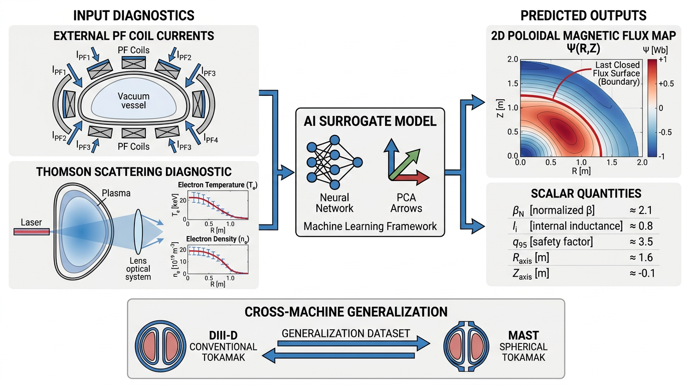
The diagnostics that built tokamak control are about to fail
Magnetic confinement fusion is transitioning from physics-exploration tokamaks to a new generation of reactor-class devices — SPARC, ARC, CFETR — designed to demonstrate net energy gain. These machines will deliver neutron fluxes more than an order of magnitude higher than any existing facility.
In that environment the very diagnostics that have underpinned tokamak control for half a century — Mirnov coils, pickup loops, Rogowski coils mounted near the vessel walls — face severe degradation. Radiation-induced EMF and conductivity produce drift voltages that exceed the signal of interest in long pulses, and structural transmutation slashes sensor lifetime to a fraction of a commercial plant’s operating hours.
The equilibrium-reconstruction problem doesn’t disappear — it becomes more important. Strip the magnetic signals from the classic EFIT code and it loses essentially all of its constraints: the capability we will most demand of next-generation devices is the one our existing toolkit cannot deliver.
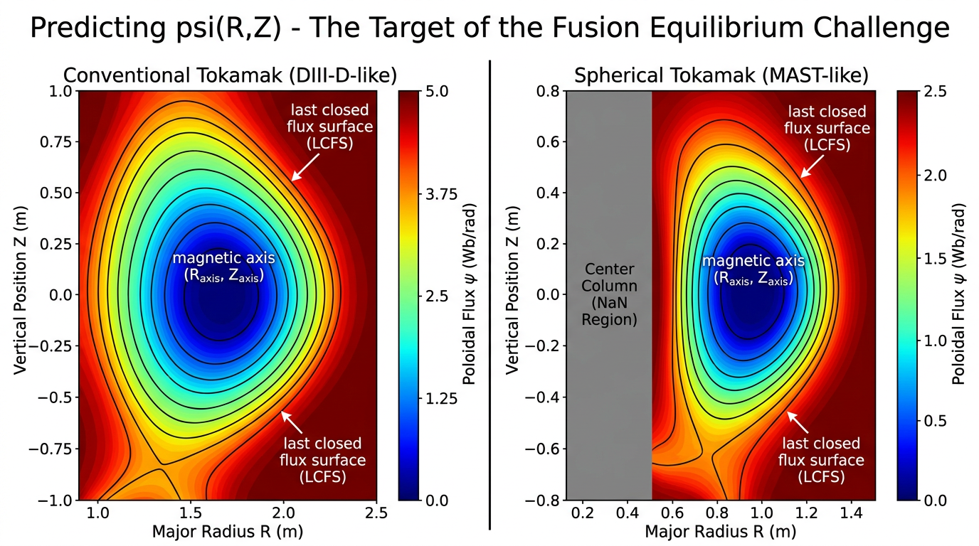
ψ(R,Z): nested contours are magnetic flux surfaces; the outermost closed surface is the plasma boundary.“Can machine learning, trained on present-day machines, learn an equilibrium representation that survives the loss of magnetic diagnostics?”
What you are given, and what you predict
For a held-out shot, you receive non-magnetic diagnostic inputs at every EFIT timestamp and predict the equilibrium.
Inputs (non-magnetic)
- Coil currents — 18 F-coils, ohmic solenoid (ECOILA) and toroidal-field coil (bcoil) on DIII-D; 10 P-coils, solenoid, toroidal-field (TF) and error-field (EFPS) coils on MAST. 21 signals on DIII-D, 14 on MAST.
- Thomson scattering — electron temperature
Teand densityneprofiles (core & edge views). - Plasma current
Ip.
Outputs (the equilibrium)
- Full flux map
ψ̂(R,Z)on a 65×65 grid — the primary target; you submit it plus two scalars (below). - Two predicted scalars — edge safety factor q95 and normalized beta βN, the only quantities a flux map cannot contain.
- Everything else is derived from your flux map — the LCFS boundary, the magnetic axis (Raxis, Zaxis), elongation and triangularity, volume, and internal inductance li are all computed from your ψ̂ by the scorer and scored for consistency with the same computation on the true ψ.
What you can win, and how
Intra-machine (DIII-D)
Reconstruct the plasma’s shape on the same machine you trained on.
- Scored on
-
S_modelS_model The composite score that decides Challenge 1:S = 0.55·R²ψ + 0.15·R²_q95,βN + 0.10·(1 − D_LCFS) + 0.20·Consistency. It blends flux-map accuracy, the two predicted scalars, boundary alignment, and the consistency of the seven ψ-derived scalars into one number in [0, 1]. Higher is better. - Wins
- Best DIII-D intra-machine reconstruction — $500
- Leaderboard
- sort by
Ch1: DIII-D S
Cross-machine (DIII-D → MAST)
Take that model to a completely different machine it has never seen — with zero training data.
- Scored on
-
G_ratioG_ratio The score that decides Challenge 2:G = S_model(MAST) / S_model(DIII-D)— the fraction of your DIII-D performance you keep when moving zero-shot to MAST. 1.0 would mean perfect transfer. It needs predictions for both machines, and only entries withS_model(DIII-D) ≥ 0.85are eligible — below that gate (or with DIII-D missing) the scorer reports 0. - Wins
- Best DIII-D → MAST cross-machine generalization — $500
- Leaderboard
- sort by
Ch2: G_ratio
Why Challenge 2 is the hard one
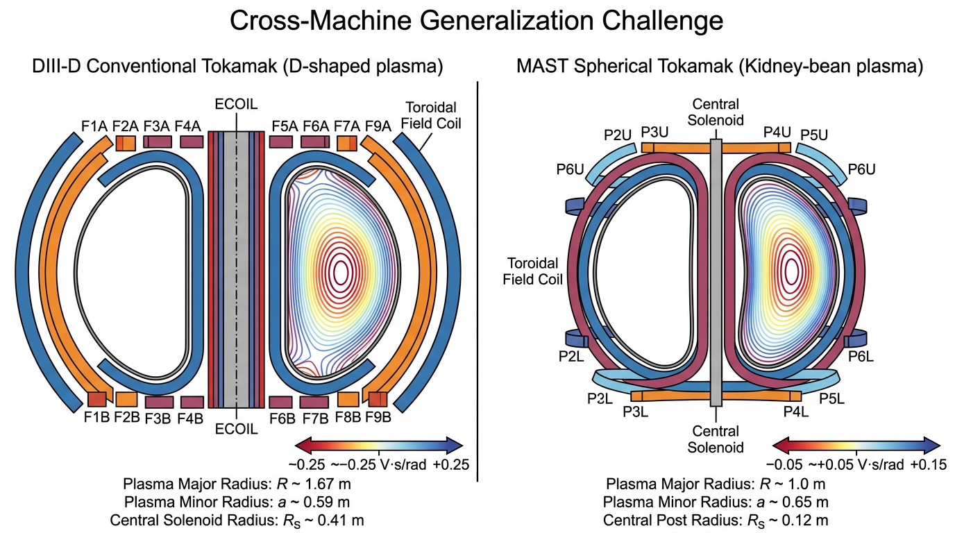
Challenge 2 asks you to train on DIII-D and transfer zero-shot Zero-shot Applying a model to a new machine with no labels from it at all. MAST has zero training shots on purpose; that is the whole of Challenge 2. Concretely: no MAST equilibrium reconstructions, from our data or any public archive, may train, fine-tune, calibrate, validate or select a MAST-predicting component. MAST inputs may be used, including unsupervised pretraining, normalization and label-free test-time adaptation. to MAST — a machine with a different shape, a different coil set, and no training data at all. Nothing about MAST is available to learn from.
Our pilot baseline makes the difficulty explicit: a naïve coil-mapping transfer scores SSIM SSIM Structural Similarity Index — an image-quality metric that rewards getting the structure right rather than each pixel exactly. Used to describe baseline results, not to score submissions. 0.83 on DIII-D but only 0.10 on MAST. We frame that collapse as a failure on purpose — it is a far more honest measure of generalization than a within-machine split, and a direct test of whether a model captures the universal physics of the Grad–Shafranov equation Grad–Shafranov equation The equation governing a tokamak equilibrium. It is the same physics on every machine — which is exactly why a model that has truly learned it should transfer from DIII-D to MAST. or merely one device’s engineering minutiae.