Get Started

From setup to first submission

Six sample shots, a desktop visualizer, and four reference baselines. Newcomers without fusion expertise can reach a working submission in well under an hour.

The path

Four steps

1 · Install

~2 min

Python with pandas, pyarrow, and plotly. That’s enough to load and plot a shot.

2 · Explore

Visual

Open a sample shot in the dFL desktop visualizer to see flux contours, coil currents, and Thomson profiles interactively.

3 · Model

Baselines

Start from a reference baseline — PCA + Ridge fits in under a tenth of a second.

4 · Submit

Codabench

Package predictions as .npz/NetCDF4 and submit to the public leaderboard.

Load a shot

Quickstart

Each Parquet file holds a single shot. The target efit_psirz is a list of 65×65 flux maps — one per efit_times slice. The two golden rules: resample inputs onto EFIT times, and never interpolate the targets.

Tutorial notebooks reproduce all four baselines end-to-end (estimated 1–2 hours from setup to first submission).

Starter Kit & Baselines (GitHub)Soon Dataset (Hugging Face)

import pandas as pd
import numpy as np

# One row per shot; every series/profile is a nested array in that row.
df = pd.read_parquet("d3d_shot_203702.parquet")

# Target: a sequence of 65x65 poloidal flux maps, one per EFIT time slice.
psirz = df["efit_psirz"].iloc[0]      # list of 2D grids
efit_t = df["efit_times"].iloc[0]     # EFIT timestamps

# Input example: an F-coil current time series (~49k samples).
f1a = np.array(df["magnetics_F1A"].iloc[0])

# Resample INPUTS onto EFIT times — never interpolate the targets.
mag_t = np.array(df["magnetics_F1A_times"].iloc[0])
f1a_on_efit = np.interp(efit_t, mag_t, f1a)

See the data

The dFL visualizer

dFL (Data Fusion Labeler) is a cross-platform desktop app for inspecting multi-rate scientific data. Point it at the challenge’s fusion_data_provider.py plugin and it auto-discovers the sample shots, then renders flux contours, Thomson heatmaps, coil currents, and the X-point gap interactively — no fusion background required.

Binaries for Apple Silicon, Windows, and Linux are published on the dFL GitHub releases page.

macOS (Apple Silicon) .dmg Windows .exe Linux .AppImage

Reference pipelines

Four baselines, simplest to deepest

All implemented in PyTorch and scikit-learn and released as Jupyter notebooks. Every one trains to within a few percent of leading numbers in under two hours on a single commodity GPU or CPU.

PCA + Ridge

<0.1 s

20-component PCA of training flux maps; RidgeCV maps the 21-dim DIII-D input to PCA coefficients. SSIM 0.84 on the demo set.

PCA + Gradient-boosted trees

Interpretable

HistGradientBoostingRegressor in a MultiOutputRegressor captures nonlinear coil coupling; inspect with SHAP.

MLP on PCA targets

MSE 0.005

3-layer fully-connected network (~41k params) over PCA coefficients — works with limited data.

Convolutional decoder

~5M params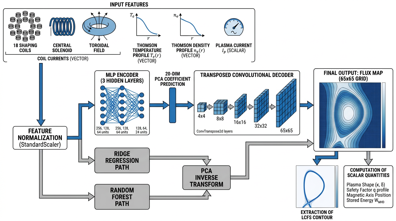

FC encoder → ConvTranspose2d upsampling to 65×65; demonstrates the capacity-vs-data tradeoff.

Output space matters more than model size. The same MLP scores MSE 0.005 on PCA targets (~41k params) but 0.239 predicting raw pixels (~5M params) on small data. Compress the target first.

Baseline architecture: inputs to PCA-compressed flux coefficients to reconstructed 65x65 map. — A representative baseline: compress the flux map with PCA, regress the coefficients, reconstruct.

Make a submission

Submission format

Package your predictions (flux maps, LCFS contours, and the five scalars) as .npz or NetCDF4 files indexed by record ID and EFIT timestamp, plus a manifest declaring which harmonization layer you used. Submit through Codabench, which scores against the hidden test set.

Submissions are capped at 5 per day and 100 total per team to discourage leaderboard probing. See Rules & Evaluation for the full scoring breakdown.

Leaderboard & Submission (Codabench)Soon Rules & evaluation →