Can AI reconstruct the magnetic geometry of a fusion plasma — without measuring the magnetic field?
That is the Fusion Equilibrium Challenge. Given only the currents in a tokamak Tokamak A doughnut-shaped machine that confines a fusion plasma with magnetic fields, combining a toroidal (the long way round) and a poloidal (the short way round) field. ’s electromagnets and a laser’s reading of the plasma, reconstruct the plasma’s hidden shape — the capability next-generation fusion reactors will need when their magnetic sensors burn out. Two challenges, two $500 awards, one open dataset.
Phase 1 (development) is open — submissions close Oct 18, 2026 · CC BY 4.0 data, MIT code.
Nested magnetic flux surfaces and helical field lines in a tokamak — rendered live. Move your cursor to orbit.
Pick your challenge — or enter both
They share one dataset, one submission format, and one leaderboard. Each is won separately, and each pays $500.
Intra-machine (DIII-D)
Reconstruct the plasma’s shape on the same machine you trained on.
- Scored on
-
S_modelS_model The composite score that decides Challenge 1:S = 0.55·R²ψ + 0.15·R²_q95,βN + 0.10·(1 − D_LCFS) + 0.20·Consistency. It blends flux-map accuracy, the two predicted scalars, boundary alignment, and the consistency of the seven ψ-derived scalars into one number in [0, 1]. Higher is better. - Wins
- Best DIII-D intra-machine reconstruction — $500
- Leaderboard
- sort by
Ch1: DIII-D S
Cross-machine (DIII-D → MAST)
Take that model to a completely different machine it has never seen — with zero training data.
- Scored on
-
G_ratioG_ratio The score that decides Challenge 2:G = S_model(MAST) / S_model(DIII-D)— the fraction of your DIII-D performance you keep when moving zero-shot to MAST. 1.0 would mean perfect transfer. It needs predictions for both machines, and only entries withS_model(DIII-D) ≥ 0.85are eligible — below that gate (or with DIII-D missing) the scorer reports 0. - Wins
- Best DIII-D → MAST cross-machine generalization — $500
- Leaderboard
- sort by
Ch2: G_ratio
Challenge 2 needs both machines. G_ratio compares your
MAST score against your DIII-D score, so an entry that predicts DIII-D only scores 0
here. Submit predictions for both to appear on that column.
The compute-light badge Compute-light badge A self-declared badge for models that train end-to-end in under two hours on a single GPU or CPU. It is a recognition that applies across both challenges — not a separate track, and not a separate leaderboard. applies to both. Train end-to-end in under two hours on one GPU or CPU and say so on your submission — it is a recognition, not a separate competition.
Two separate steps: registering here puts you on the announcements list; joining on Codabench is what lets you submit and be scored.
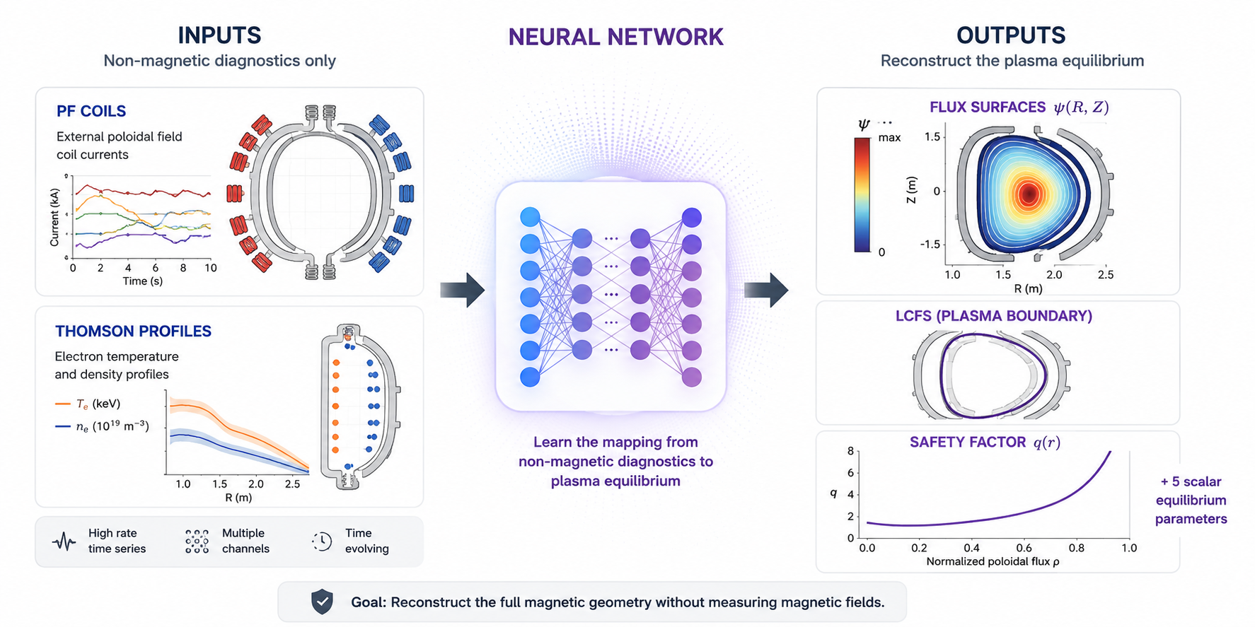
From non-magnetic diagnostics to the full equilibrium
A single learned mapping turns coil currents and laser profiles into the flux surfaces, plasma boundary, and equilibrium parameters EFIT normally derives from magnetic sensors.
Explain it like I’ve never seen a tokamak
Imagine baking a cake in an oven you can’t open. You can’t see or touch it — but you can read the dials. Your job: predict exactly what the cake looks like inside. That’s this challenge.
A few dozen sensor signals
The dialsNoisy time series
MessyA 2D field to rebuild
The cakeNo fusion background required — the FAQ & glossary explain every term, and four reference baselines get you from zero to a first submission fast.
Future fusion reactors such as SPARC and ARC may not be able to rely on traditional magnetic diagnostics, because intense neutron radiation degrades the sensors. Reliable, AI-based equilibrium inference could therefore become a core component of reactor control systems — making this challenge a rehearsal for a capability real power plants will need.
From diagnostics you can keep, to the field you can’t measure
Strip away the magnetic sensors and the classic EFIT reconstruction loses its constraints. Can machine learning, trained on today’s machines, learn an equilibrium that survives without them?
① Inputs you’re given
Non-magneticIp Ip (plasma current) The total electric current flowing through the plasma itself — of order 10⁶ A, roughly 100× the coil currents. Given as an input. .
② Your model
Any method③ What you predict
ψ + 2 scalarsψ(R,Z) Poloidal flux ψ(R,Z) The 2D field you are asked to predict. Its contour lines are the magnetic surfaces that hold the plasma in place — so a map of ψ is effectively a picture of the plasma’s shape. plus just
q95 q₉₅ (edge safety factor) How many times a magnetic field line goes the long way round the torus for each time it goes the short way, measured near the plasma edge. It is a stability margin — hence "safety". One of the two scalars you submit (it depends on the toroidal field function, which a flux map cannot contain). and βN β_N (normalized beta) How much plasma pressure the magnetic field is holding, normalized so machines of different sizes can be compared. One of the two scalars you submit (it depends on the pressure profile, which a flux map cannot contain). . The boundary
( LCFS LCFS Last Closed Flux Surface — the outermost magnetic surface that closes on itself without hitting a wall. In practice: the edge of the plasma. ), magnetic axis, shape, volume and li l_i (internal inductance) A measure of how peaked the electric current is across the plasma — high l_i means current concentrated in the core. You do not submit it: the scorer derives l_i from your flux map (part of the Consistency term). are
all derived from your flux map by the scorer — your ψ has to earn them.
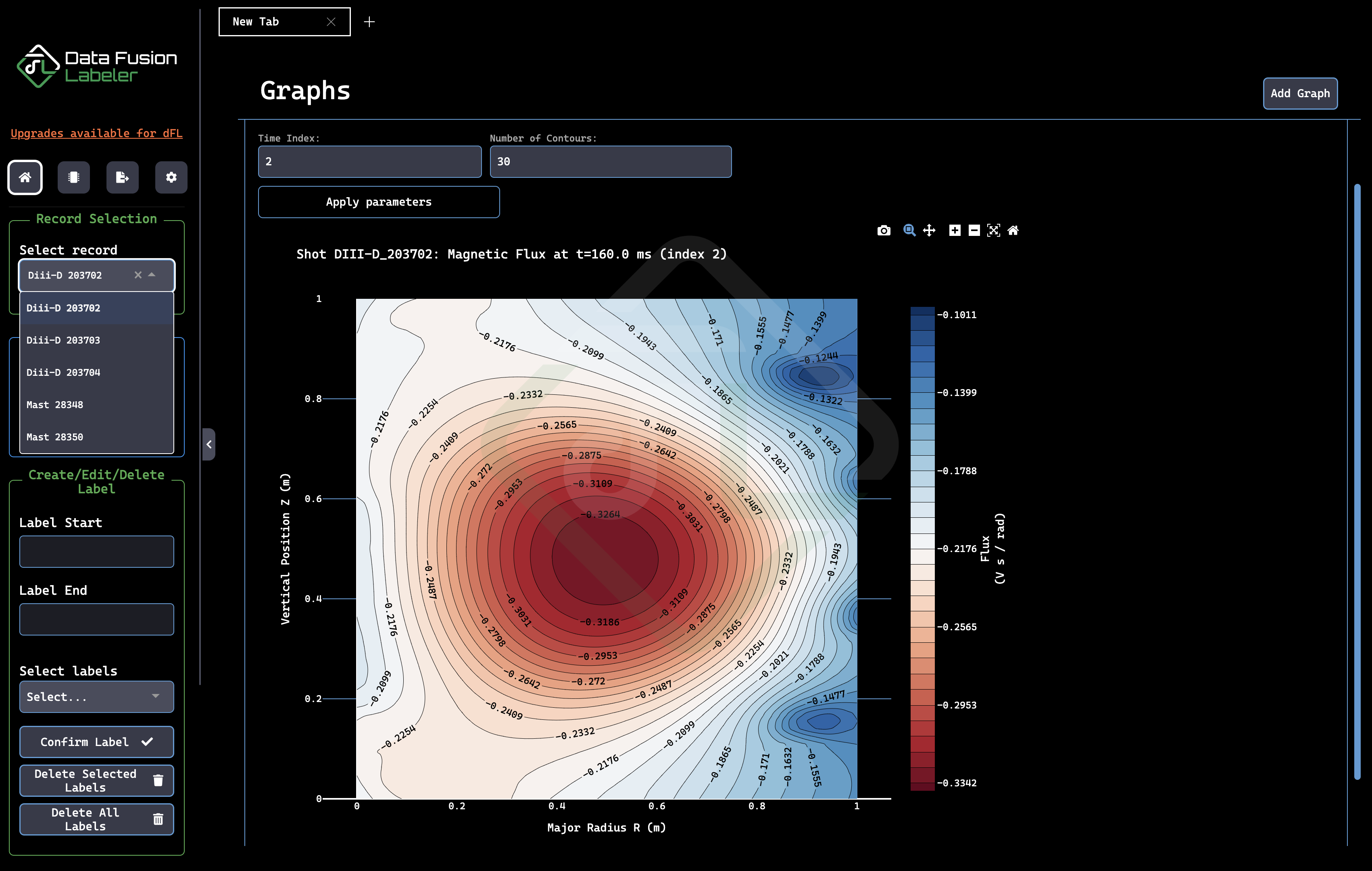
What a shot looks like in the dFL visualizer
The free Data Fusion Labeler desktop app renders every shot — flux contours, Thomson profiles, and coil-current traces — so you can sanity-check inputs and confirm your pipeline before you train.
The cross-machine generalization stress test
Train on DIII-D, transfer to MAST. A naïve coil-mapping baseline collapses from SSIM 0.83 to 0.10 — an honest measure of whether a model learns the universal Grad–Shafranov physics or just one machine’s quirks.
| DIII-D (conventional) | MAST (spherical) | |
|---|---|---|
| Type | Conventional tokamak (D-shaped) | Spherical tokamak (low aspect ratio) |
| Facility | DIII-D · General Atomics, San Diego | MAST · UKAEA Culham, UK |
| Shots (released set) | 7,915 | 1,206 |
| Training data | 7,041 shots | None — zero-shot by design |
| Target flux grid | 65 × 65 | 65 × 65 |
| Shaping coils | 18 F-coils (F1A–F9B) + ECOILA, bcoil | 10 P-coils (P2L–P6U) + sol, tf, efps |
| Magnetics time base | Shared magnetics_time, length varies by shot (480k @ 20 kHz, or ~49k @ 2 kHz); Ip on its own ADC | Shared magnetics_time (~30k samples) |
| Typical flux value | ≈ −0.25 V·s/rad | ≈ +0.05 V·s/rad |
We include the DIII-D → MAST test to measure whether a model has captured the transferable physics of the equilibrium rather than one device’s quirks. That property is what would let future reactors be designed and optimized from data long before they exist, with no real shots to learn from — and short of that ideal, it still yields a warm start for fine-tuning on a new machine’s first campaigns instead of beginning from zero.
Two phases: develop in the open, then a blind final
- Jul 2026 Complete
Public release of training & public test data
- Jul 27 – Oct 18, 2026
Phase 1 (development) — continuous public leaderboard
- Oct 19, 2026
Blind test data released; Phase 2 (final) opens
- Oct 26, 2026
Phase 2 (final) closes — last call for submissions
- Dec 2026
NeurIPS competition session & results
Phase 1 — development
Jul 27 – Oct 18, 2026Phase 2 — final (blind)
Oct 19 – Oct 26, 2026Beyond the two $500 awards: four honorable mentions, named co-authorship on the lessons-learned paper, and invited NeurIPS talks.
Built with the fusion community
 Sophelio
  DIII-D / General Atomics
  UKAEA · MAST-U
  University of Texas at Austin
 Ready to infer what you cannot measure?
Six sample shots, a desktop visualizer, and four reference baselines get you from setup to a first submission in well under an hour.