How submissions are scored
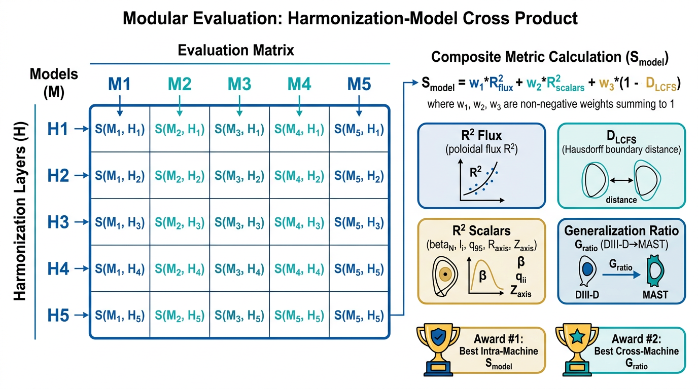
Four metrics combine into one composite score. Challenge 1 ranks on that score; Challenge 2 ranks on how much of it you keep when you move to a new machine.
What we measure
Flux accuracy
Coefficient of determination of the predicted flux map over all grid points, timesteps, and test shots. The primary signal of reconstruction quality.
Predicted scalars
Mean R² of the only two scalars you submit — q95 q₉₅ (edge safety factor) How many times a magnetic field line goes the long way round the torus for each time it goes the short way, measured near the plasma edge. It is a stability margin — hence "safety". One of the two scalars you submit (it depends on the toroidal field function, which a flux map cannot contain). and βN β_N (normalized beta) How much plasma pressure the magnetic field is holding, normalized so machines of different sizes can be compared. One of the two scalars you submit (it depends on the pressure profile, which a flux map cannot contain). . They are the two equilibrium parameters that a flux map cannot contain (they need the toroidal field function and the pressure profile), so they remain genuine prediction targets.
Boundary alignment
Symmetric Hausdorff distance Hausdorff distance The worst-case gap between two shapes: how far you must travel from the least-well-matched point on one contour to reach the other. Used to compare predicted and true plasma boundaries. between the predicted and true LCFS LCFS Last Closed Flux Surface — the outermost magnetic surface that closes on itself without hitting a wall. In practice: the edge of the plasma. contours, normalized by the true LCFS major radius. Smaller is better. You do not submit a contour — the scorer extracts it from your flux map.
ψ-derived scalars
Mean agreement of seven scalars the scorer derives from your submitted flux map — Raxis, Zaxis, elongation κ, triangularity δtop/δbot, volume V, and li l_i (internal inductance) A measure of how peaked the electric current is across the plasma — high l_i means current concentrated in the core. You do not submit it: the scorer derives l_i from your flux map (part of the Consistency term). — scored against the same derivation on the true flux. A scalar can only be earned by a flux map that implies it.
No scalar is skipped because of boundary type. The corpus is
diverted-only, so the
limited-plasma carve-out that used to exclude the shape terms is gone. A frame leaves a scalar's
average only when the ground-truth derivation itself fails on it — a degenerate frame with
no closed flux surface, say. If your flux map fails to yield a scalar the truth does have,
that is not a free pass: the scorer substitutes the mean and you take the loss. A perfect flux map
scores D_LCFS = 0 and Consistency = 1 by construction, because the same
published code runs on your flux and on the true flux.
One score per challenge
S_model S_model The composite score that decides Challenge 1: S = 0.55·R²ψ + 0.15·R²_q95,βN + 0.10·(1 − D_LCFS) + 0.20·Consistency. It blends flux-map accuracy, the two predicted scalars, boundary alignment, and the consistency of the seven ψ-derived scalars into one number in [0, 1]. Higher is better.
S = 0.55·R²ψ + 0.15·R²_q95,βN + 0.10·(1 − D_LCFS) + 0.20·Consistency
Highest composite S_model on the hidden DIII-D test set.
G_ratio G_ratio The score that decides Challenge 2: G = S_model(MAST) / S_model(DIII-D) — the fraction of your DIII-D performance you keep when moving zero-shot to MAST. 1.0 would mean perfect transfer. It needs predictions for both machines, and only entries with S_model(DIII-D) ≥ 0.85 are eligible — below that gate (or with DIII-D missing) the scorer reports 0.
G = S_model(MAST) / S_model(DIII-D)
Highest G_ratio among entries reaching a DIII-D composite S_model ≥ 0.85 (gate enforced by the scorer).
S_model is a weighted blend in [0, 1] — R² terms are clipped at 0 and
D_LCFS at 1. G_ratio is the fraction of your DIII-D performance retained under
zero-shot Zero-shot Applying a model to a new machine with no labels from it at all. MAST has zero training shots on purpose; that is the whole of Challenge 2. Concretely: no MAST equilibrium reconstructions, from our data or any public archive, may train, fine-tune, calibrate, validate or select a MAST-predicting component. MAST inputs may be used, including unsupervised pretraining, normalization and label-free test-time adaptation. transfer, so values near 1 mean near-complete transfer. Because it is a
ratio of the two, Challenge 2 requires predictions for both machines: a
DIII-D-only entry scores G_ratio = 0.
Submission format
What the scorer expects
.npz per machine, keyed by shot and EFIT timestamp: your flux maps plus
q95 and betaN — nothing else. The boundary, axis, shape, volume and
li are all derived from your flux map by the scorer.
Scoring runs CPU-only, well within the platform limit.
The manifest
manifest.json travels with your predictions. It is descriptive only — the scorer
locates your predictions by filename, so keep the two .npz named exactly
as the config names.
Development, then a blind final
Phase 1 — development
Jul 27 – Oct 18, 2026Phase 2 — final (blind)
Oct 19 – Oct 26, 2026Rules & eligibility
- 1 Each team joins the competition on Codabench with a single valid contact email; aliases that already exist as solo participants are deactivated. Registering with the organizers is a separate step and is not required to be scored.
- 2 External public datasets (other tokamak archives, OMFIT-produced equilibrium tables) and publicly available pre-trained vision or scientific foundation models are permitted, with explicit disclosure in the methods report. See rule 3 for the one exception.
- 3 No MAST equilibrium data. Equilibrium reconstructions of MAST or MAST-U from any source — the FAIR-MAST archive, mirrors of it, datasets derived from it, or model weights trained on it — may not be used to train, fine-tune, calibrate, validate or select any model or component that produces MAST predictions, including hyperparameter search and checkpoint selection. This covers flux maps, LCFS contours, EFIT-derived scalars, and aggregates of them such as bases or priors. Permitted and unaffected: MAST inputs used without targets (including self-supervised pretraining, target-domain normalization, distribution alignment and label-free test-time adaptation), MAST machine geometry, equilibria from other machines, and synthetic equilibria from your own free-boundary solver calibrated against MAST inputs. The three labelled MAST demo shots are for format inspection and visualization only. The competition's own feedback is not covered: the scores and Detailed Results the Development phase returns for your submissions may be used to compare, tune and select MAST pipelines, and that use must be stated in the methods report. The line is whether you can score against MAST equilibria yourself, offline — that is barred; the scores the platform returns for a submission are not. Probes are not feedback: a submission built to measure the labels rather than to be judged as a candidate (for example a constant, shifted or rescaled prediction) reveals label statistics, and those statistics — and any constant fitted to them or chosen by computing scores offline from them — count as MAST equilibrium data. The starter kit's fusion_scoring/masks/mast_envelope.npz is a union of MAST LCFS contours: use it only inside the official scoring derivation, never as a model input, feature, loss mask or prior. Effective 2026-09-23 (feedback clause 2026-10-01; probe and mask clauses 2026-10-04); Development-phase entries are not judged retroactively.
- 4 No restriction is placed on programming language or framework. AI coding assistants may be used for any part of an entry, provided the workflow is disclosed in the methods report and the entrant takes responsibility for the submission.
- 5 All train/test splits must respect shot-level boundaries.
- 6 Every Final-phase submission must be accompanied, at submission time, by a reproduction package reference: a Git repository at a pinned commit SHA on any public forge, or a versioned archive on any public host identified by its SHA256. The package must contain model source, a pinned environment specification, the trained weights used for the submission, a training entrypoint that rebuilds the model from scratch, an inference entrypoint, and a data-provenance statement per machine. Training must be reproducible within 24 GPU-hours on a single 80 GB A100-class GPU or equivalent. Only GPU work counts toward that ceiling: CPU-only data generation (for example synthetic equilibria from your own solver) must be declared with its hardware and wall-clock but is not capped, and the package may ship the generated data with SHA256 checksums for the rebuild to start from, provided the code that generates it is included. Organizers rebuild the top five entries per challenge.
- 7 Top three teams in each award category must release source code under an OSI-approved licence and submit a 1–2 page methods report before prizes are paid.
- 8 Organizing-team members with access to the hidden ground truth are excluded from prize eligibility.
- 9 All participants follow the NeurIPS Code of Conduct.